Fun facts about large learning rates: how large is large, and what tricks they can do?
Background
Gradient Descent
Machine learning models are often trained by 1st-order optimizers, which are methods that use 1st derivative information to iteratively search the minimum of an objective function. Gradient Descent (GD) is a central one of these optimizers, and even though many results can extend beyond GD, we will focus on GD in this expository blog. GD uses iteration \[ x_{k+1}=x_k - h \nabla f(x_k) \] where $h$ is the learning rate (LR for short; numerical people also call it stepsize).
The nice classical regime of learning rates
Some functions enjoy a nice property called smoothness (in CS/optimization terminology), and understanding the convergence of GD is the easist for smooth $f$. Specifically, $f$ is $L$-smooth if $\nabla f$ is globally Lipschitz with coefficient $L$. This is a strong assumption (e.g., $f(x)=x^2$ is 2-smooth, but $f(x)=x^4$ is not smooth in $\mathbb{R}$), and it sometimes can be relaxed (e.g., one can make it local, or use prior knowledge of a bounded domain) but let’s first see what it can do.
Thm. If $f$ is $L-$smooth, $\min f$ exists, and $h<\frac{2}{L}$, GD converges to a stationary point.
Proof. Let $\min f=f^*$. \[ f(x_{k+1})\le f(x_k)+\langle\nabla f(x_k),{x_{k+1}-x_k}\rangle+\frac{L}{2}|x_{k+1}-x_k|^2 =f(x_k)-h(1-\frac{L}{2}h)|\nabla f(x_k)|^2. \]
Then \[ \sum_{k=1}^N|\nabla f(x_k)|^2\le \frac{1}{h(1-\frac{L}{2}h)}(f(x_0)-f(x_N)) \le \frac{1}{h(1-\frac{L}{2}h)}(f(x_0)-f^*). \] Therefore $\lim_{k\to\infty}|\nabla f(x_k)|^2=0$, i.e., GD converges to a stationary point.
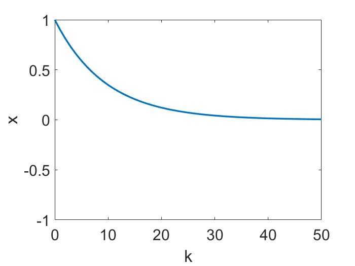
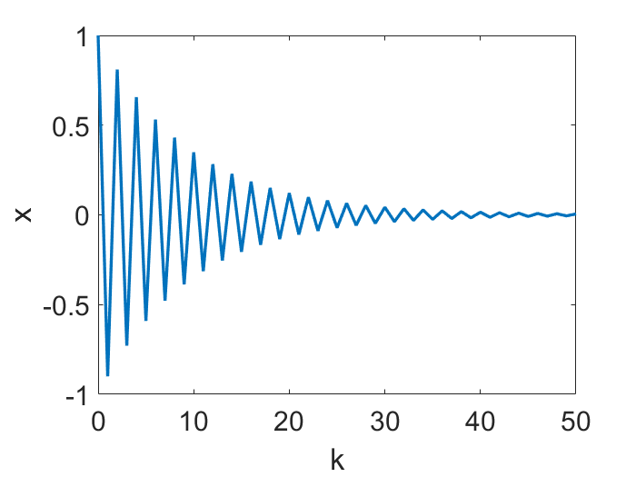
Therefore, $h<2/L$ is a nice regime. One fun thing to note though, is that this regime can be further divided. As the following animations show (for a simple $f=x^2/2$), $h<1/L$ leads to continuous motion of $x_k$, but a bigger $h$ gives a discontinuous, oscillatory behavior, however only in $x_k$ but not in $f(x_k)$!
Nice part of the nice regime, and gradient flow
A computational mathematician would immediately recognize gradient descent as a forward Euler discretization of the gradient flow ODE \[ \dot{x}=-\nabla f(x) \] Obviously in this continuous time / infinitesimal $h$ limit, $x$ is changing continuously. It will be fun to connect to classical numerical analysis and explore where the $h<1/L$ condition mentioned above comes from! It makes gradient descent close to gradient flow. We shall call $h$ such that gradient descent approximates gradient flow small LR.
However, the larger $h$ becomes, the more GD deviates from gradient flow. Obviously, the oscillatory behavior at $1/L < h < 2/L$ deviates significantly from gradient flow.
ODE beyond gradient flow?
Backward error analysis, a.k.a. modified equation
Gradient flow only captures the behavior of GD when $h$ is sufficiently small. However, ODE can still help gain insight of GD when $h$ is larger. How is this possible, given that the gradient flow ODE is the $h\to 0$ limit of GD? The answer is, just like Taylor expansion, one can add $\mathcal{O}(h), \mathcal{O}(h^2), \cdots$ terms to the ODE to correct for the finite $h$ effect.
How to precisely do this has been well developed in numerical analysis under the name “backward error analysis”, and the corrected ODE is called “modified equation”. The seminal idea dates back to at least [Wilkinson (1960)] and the subject is beautifully reviewed, for example, in [Hairer, Lubich and Wanner (2006)].
Now let’s apply this general tool to the specific case of GD. Doing it to 1st-order in $h$ gives \[ \dot{x}=-\nabla f_1(x), \text{ where } f_1(x):=f(x)+\frac{h}{4}|\nabla f(x)|^2_2\] and it approximates GD in the sense that $x(kh)\approx x_k$, just that for gradient flow (a 0th-order approximation, $f_0:=f$). In this case, the 1st-order modified equation is still a gradient flow, and $f_1$ is thus called a (1st-order) modified potential.
Discussions
The 1st-order modified potential $f_1$ is useful. For example, it can characterize some implicit bias of GD as a modification of landscape, and as in 2022 the community continues to find its exciting machine learning implications. However, the methodology is not new.
In fact, obtaining the expression of $f_1$ is relatively easy, simply by matching the GD iterate with the Taylor expansion of $x(h)$ in $h$. This “derivation” however is only formal, and it might even give a false impression that this works for any $h$. However, a power series (in $h$) has a radius of convergence, and its generalization to an ODE will have a similar issue of convergence. A beautiful paper, [Li, Tai and E (2019)], went beyond a formal series matching. Instead, it rigorously characterized the accuracy of 1st-order modified equation when $h$ is small enough. Its setup is also more general (SGD), which includes GD as a special case. The modified equation for exactly the GD case was also explicitly provided in the literature. For example, [Kong and Tao (2020)] quantitatively discussed when/how/why $f_1$ is insufficient, and of course $f_1$’s expession was provided, even though that was not the point of their paper.
Indeed, $\dot{x}=-\nabla f_1(x)$ can approximate GD for $h$ values larger than those for $\dot{x}=-\nabla f(x)$, but if $h$ becomes too large, it will lose all its approximation power.
Will higher-order modified equation help with large $h$? In most cases, no. In fact if $h$ is too large, higher-order modified equation (i.e. more correction terms) may even lead to worse approximation.
These facts can be exemplified by the following plots, where the LR is respectively 1) small so that gradient flow is a good approximation; 2) still $<1/L$, but medium so that gradient flow is insufficient but modified equation is a good approximation; 3) larger, $\in (1/L, 2/L)$, and modified equation no longer works well; 4) truly large, $>2/L$, and for this simple objective function ($f=x^2/2$) GD blows up.
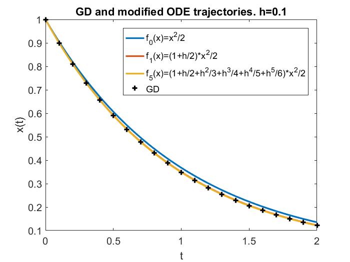
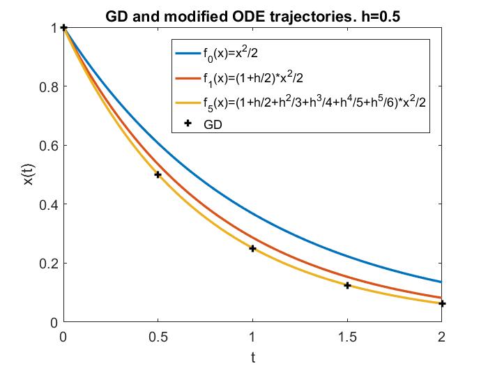
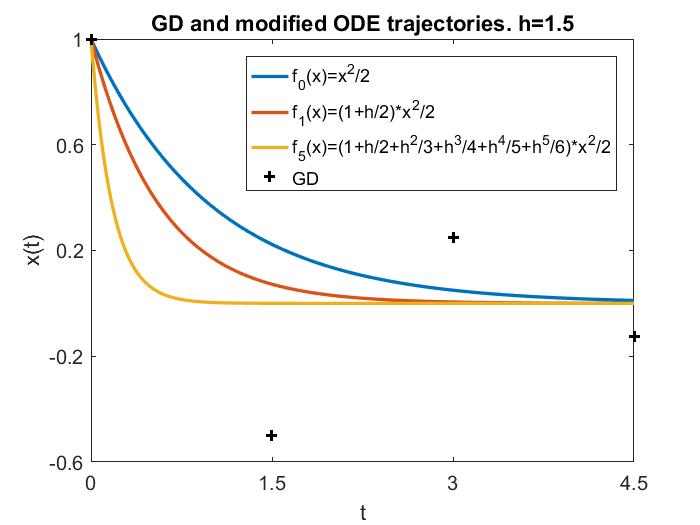
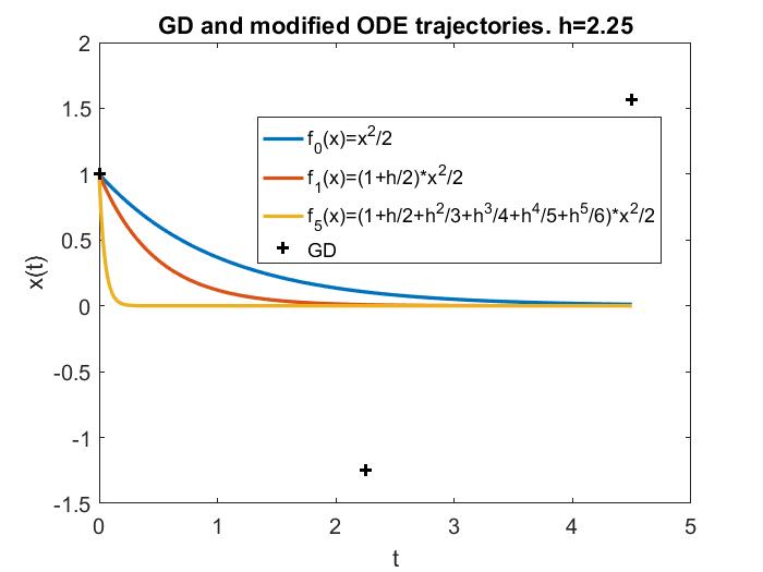
A remark is, although some literature use modified equation to study “large” LRs, for consistency, throughout this blog we will call such LRs medium instead, because there are larger LRs for which modified equation completely breaks down, and yet GD may still work and produce nontrivial and very interesting behaviors, which oftentimes are beneficial to deep learning.
Truly large learning rates
Now let’s exemplify some of the aforementioned behaviors of truly large LR.
Welcome to the zoo
Nonconvergence. The first instinct one might have is, if LR is too large, GD will just blow up (i.e. iterates grow unboundedly). This indeed could happen, such as whenever $h>2/L$ for quadratic objectives, as illustrated below (again for a simple $f=x^2/2$):
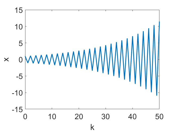
However, for more complex $f$’s, GD does not necessarily blow up under large LR.
Nor does GD always converge to a point, when convergent! We can view the gradient descent iteration as a discrete-in-time dynamical system. It is known that dynamical systems can have attractors of various sorts, some most common ones being fixed point, periodic orbit, and strange attractor (yes, we’re speaking about chaos). And they all can show up in GD dynamics!
Periodic orbits. Figures below are examples of periodic motions produced by GD for a miniature matrix factorization problem, with $f(x,y)=(1-xy)^2/2$ (note: seemingly simple, but in fact not $L$-smooth for any $L$, nor convex). Various values of period are possible, but in none of these figures is the convergence to any minimizer.
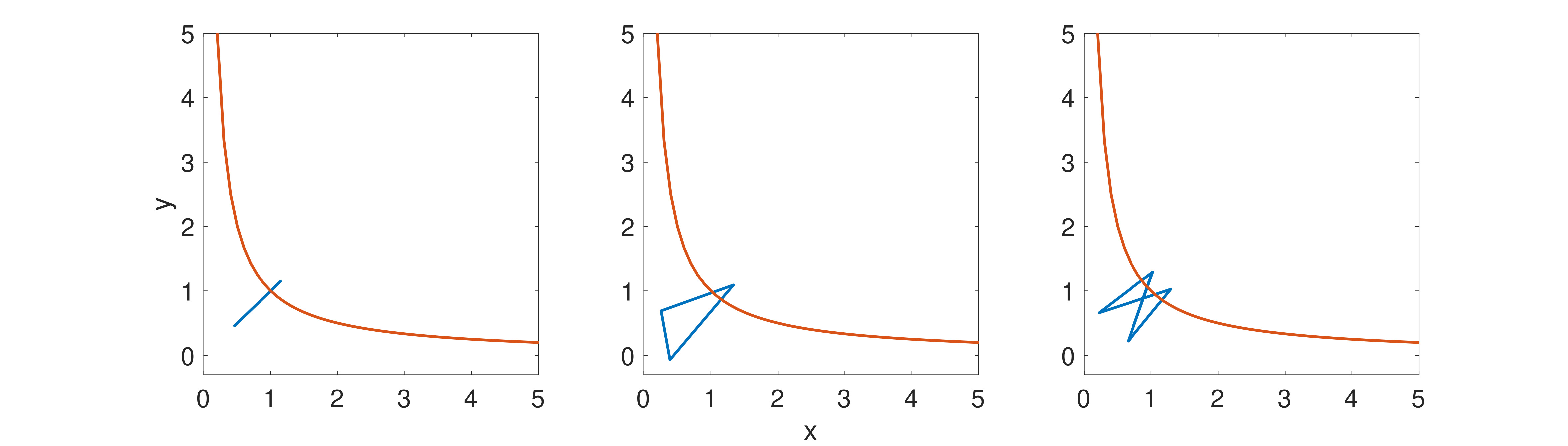
GD with h=1.9 converges to three orbits with period 2, 3 and 4 respectively (depending on initial condition). Blue lines are the orbits; red line is a reference line of all minima xy = 1.
These figures are from [Wang et al (2022)], although not the main points of that article. More will be discussed in the 2nd next section.
Strange attractor. Let’s now take a look at a case of convergence to a chaotic attractor, a famous example of which is the Lorenz butterfly.
These figures are from [Kong and Tao (2020)]. Again, more will be explained, right below:
An alternative mechanism for escapes from local min
The energy landscape in the above animation has a lot of (spurious) local minima. Impressively (but also rather intuitively), GD iterations can jump out of these local minima, as animated.
This is actually due to a large LR! In fact, if the LR were instead small, GD would just converge to a local minimum close to its initialization, just like gradient flow.
People recently started to appreciate this effect of large learning rate, and empirical results gradually appeared in the literature. A major reason is that the deep learning community, for example, is very much interested in escapes from local minima, which often correspond to improved training accuracy. The most popular mechanism for local min escape is via noise, which usually originates from stochastic gradients. Large LR, however, is a completely complementary escape mechanism, as it requires no stochasticity. A quantitative and rigorous analysis, however, was already provided in [Kong and Tao (2020)], and its main idea will now be sketched:
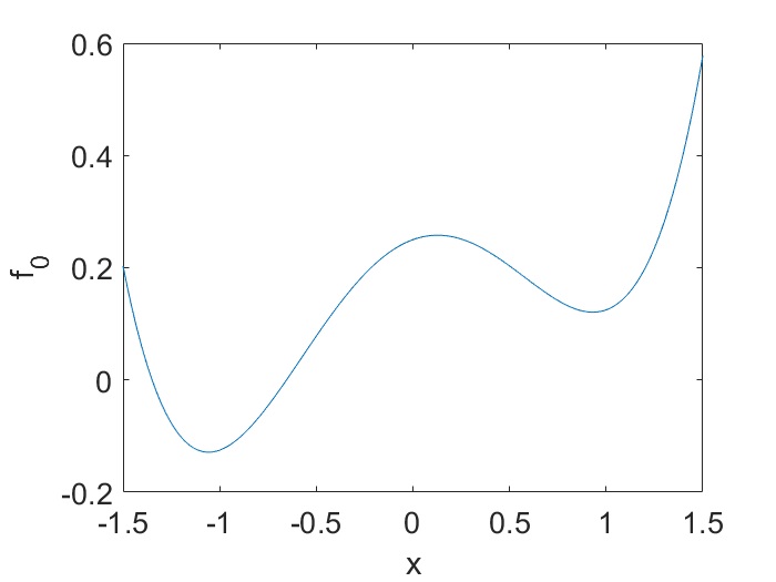
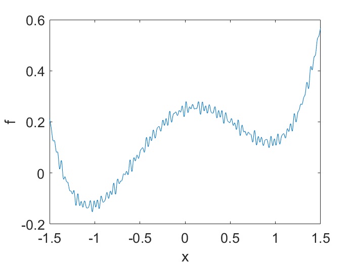
Given the objective function $f$, let’s decompose it as $f(\textbf{x})=f_0(\textbf{x})+f_1(\textbf{x})$, where $f_0$ corresponds to macroscopic behavior and $f_1$ encodes microscopic details, such as illustrated by the following 1D example:
When LR becomes large enough, it is no longer able to resolve the details of $f_1$. This is just like if you drive very fast, small pebbles and bumps on the road can no longer be felt. What is “large enough”? Denote the microscopic scale (when compared to the macroscopic scale) by $\epsilon$ and suppose $f_1$ is $L$-smooth, then $L=\mathcal{\Omega}(1/\epsilon)$ due to 2nd-order spatial derivative, which means traditional small LR is $h=o(1/L)=o(\epsilon)$. If $h=o(1)$ instead, independent of $\epsilon$, then $h\gg 1/L$, and it is large enough.
Using this setup, [Kong and Tao (2020)] rigorously proved that the microscopic part of the gradient, $-h\nabla f_1(\textbf{x})$, effectively acts like a noisy forcing to the deterministic GD dynamics. In fact, using tools from dynamical systems, probability, and functional analysis, they proved that the GD iterates actually converge to a chaotic attractor, and hence to a statistical distribution, which is very close to \[ Z^{-1} \exp(-f_0(\textbf{x})/T)d\textbf{x} \] under reasonable assumptions. Those familiar with statistical mechanics can immediately recognize this approximate distribution as the famous Gibbs distribution. Rather notably, this distribution, being the limit of GD, only depends on the large scale part of the objective, $f_0$, and small details encoded by $f_1$ are not even seen anymore, as a consequence of a large LR ($h\gg 1/L$)!
This quantitative result also suggests that smaller values of $f_0$ (and $f$ too) will have (significantly) higher probability, which roughly means they will be visited more often after many GD iterations. This is usually desirable (smaller training loss, likely beneficial for test accuracy as well), and thus a benefit of large LR.
In these senses, large LR GD behaves very much like SGD, even if there is no randomization or minibatch. It thus provides an alternative means of escape from minima.
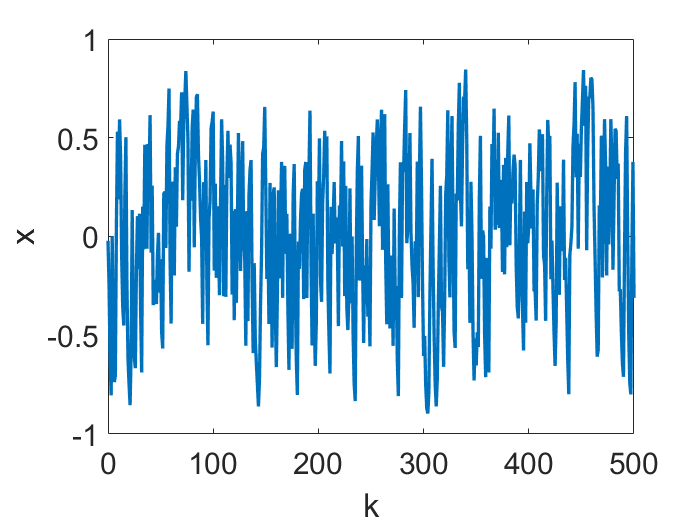
A lot more details can be found in [Kong and Tao (2020)], but here is a final excerpt: do objective functions in real problems admit such multiscale structures? Both theoretical and empirical discussions were given in their paper. For example, if training data is multiscale, it is theoretically possible that the loss of a neural network, for regressing the data, inherits a multiscale structure! Here is what GD iterations give for an examplary weight parameter during training a small feedforward network:
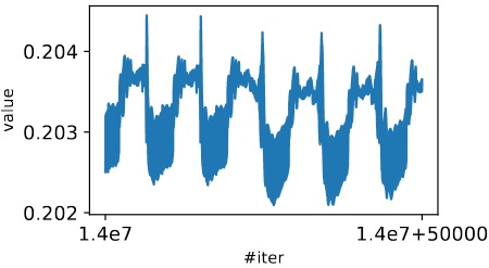
You see it doesn’t converge to any single value, but rather “blobs”, whose concatenation is actually (the projection / marginal support) of a chaotic strange attractor / probability distribution.
TL;DR [Kong & Tao (2020)] show that GD can, with the help of large LR, escape local minima and exponentially prefer small objective values, because in this case GD is actually sampling a statistical distribution, instead of merely optimizing the objective. This is due to chaotic dynamics created by large LR.
An implicit bias of large LR: preference of flatter minima
Now let’s go back to the simple case, namely the convergence of GD to a single point. Even this simple case is not simple at all, but much fun. We will just discuss one example, namely a rigorous proof of preference of flatter minima, enabled by large LR. But first of all, why do we care?
Popular Conjecture 1: Flatter minima generalize better.
There are many work arguing for this belief, while interesting results showing the contrary also exist. We do not intent to say anything new here, but only hope it is meaningful to find flatter local minima.
Popular Conjecture 2: Large LR helps find flatter minima.
This conjecture is much more recent, but due to its importance, attention is rapidly building up in the literature. Not only did empirical results emerge, but also semianalytical work, such as those based on the $\mathcal{O}(h)$ correction term in 1st-order modified potential $f(x)+\frac{h}{4}|\nabla f(x)|^2_2$ (see above section “Backward error analysis, a.k.a. modified equation”).
[Wang et al (2022)] went beyond medium LRs for which modified potential works, and studied large LRs, for which the preference of flatter minimum is even more pronounced. They provided a rigorous proof of Popular Conjecture 2, for a subclass of problems.
More precisely, consider a matrix factorization task formulated as an optimization problem \[ \min_{X,Y}~ \frac{1}{2} |A-XY^\top|^2,\quad \text{where}\ A\in\mathbb{R}^{n\times n},\ X,Y\in\mathbb{R}^{n\times d}. \] where one tries to find a rank $d$ approximation of $n\times n$ matrix $A$. This is a rather general and important data science problem per se, but for those interested in deep learning, it is also almost the same as the training of a 2-layer linear neural network.
The landscape of $f(X,Y):=\frac{1}{2} |A-XY^\top|^2$ is intriguing. For example, 1) minimizers are not isolated or countable; in fact, if $(X,Y)$ is a minimizer, so is $(cX,Y/c)$ for any constant scalar $c\ne 0$. The authors call this property homogenity, and it persists even if certain nonlinear activations are applied, for example for $\frac{1}{2} |A-X\sigma(Y^\top)|^2$ where $\sigma$ is ReLU or leaky-ReLU. 2) each local minimizer is a global minimizer.
However, amongst the minimizers some are flat and some are sharp. In fact, one could compute eigenvalues of the Hessian of $f$ and evaluate at a minimizer. Then it will be seen that $|X|\approx|Y|$ means the landscape is flat locally around the minimizer, and having unbalanced norms implies sharp local geometry instead.
Besides possible deep learning implications (flat means better generalization (?)), having flatter geometry also benefits both analysis and numerical performance of GD (otherwise smaller LR is needed). That’s why the literature oftentimes add explicit regularizers to $f$ to promote balanceness.
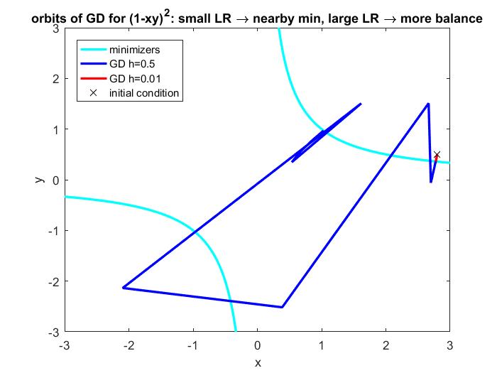
[Wang et al (2022)] showed that, if the LR is large enough, GD will start to pick minimizers with balanced norms. Moreover, the larger LR is, the more balance GD can create. No regularizer is needed. Here is a visualization based on a simplest example; see how GD can travel afar to gain balance (and hence flatness) via large LR, even when the initial condition is already close to an unbalanced minimizer and small LR simply takes you there.
(Side remark: in a way, [Wang et al (2022)] can also be thought as related to a phenomenon known as Edge of Stability that was empirically discovered recently [Cohen et al (2021)] and starting to attract attention.)
More precisely, what [Wang et al (2022)] proved include: 1) if convergent to a point, GD with large enough $h$ has an implicit regularization effect of balancing, and the limiting point $(X_\infty,Y_\infty)$ of GD iterates will satisfy a bound of $|X_\infty-Y_\infty|$ that decreases with $h$. 2) GD with large $h$ converges. The first sounds mouthful but important, and the second sounds easy; however, the truth is, 1) can actually be obtained using existing dynamical systems tools in an intuitive way, but 2) is much more nontrivial to obtain. This is all because of large LR. Advanced readers might find the proof fun and appreciate the in-depth scrutinization of GD dynamics, but details won’t be loaded here.
However, there is (again) an important point pertinent to this blog — how large is large? Very roughly speaking, the regime where balancing is pronounced is $h\in (2/L,4/L)$, which defies traditional tools briefly reviewed in the beginning of this blog. Note also that bigger $h$ can make GD not convergent.
Expert readers may ask, hold on, what is $L$? In fact, the objective function is quartic (i.e. a 4th-order polynomial) and its gradient is not globally Lipschitz. The merits of the dynamical analysis lie in not only the fact that $h>2/L$, but also that it requires only local Lipschitzness. The $L$ in $(2/L,4/L)$ is simply the spectral radius of Hess$f$ at initialization.
TL;DR [Wang et al (2022)] show that GD has, when the LR is truly large, an implicit regularization effect of converging to flatter local min. Larger LR makes the implicit bias stronger.
Thank you for reading
That’s it for this blog, which is just the tip of an iceberg. For the sake of length and the diversity of readers, there are a lot of rigor and details, as well as related work, that are omitted and sacrificed. But questions and comments are always welcome. We hope you liked it, and please feel free to cite!
Acknowledgement
We thank Tuo Zhao for encouraging us to write a blog.
References
[1]: J.H.Wilkinson. Error analysis of floating-point computation. Numer. Math. 1960
[2]: Ernst Hairer, Christian Lubich, and Gerhard Wanner. Geometric Numerical Integration. Springer 2006
[3]: Qianxiao Li, Cheng Tai, and Weinan E. Stochastic modified equations and dynamics of stochastic gradient algorithms i: Mathematical foundations. JMLR 2019
[4]: Lingkai Kao and Molei Tao. Stochasticity of deterministic gradient descent: Large learning rate for multiscale objective function. NeurIPS 2020
[5]: Yuqing Wang, Minshuo Chen, Tuo Zhao, and Molei Tao. Large Learning Rate Tames Homogeneity: Convergence and Balancing Effect. ICLR 2022
[6]: Jeremy Cohen, Simran Kaur, Yuanzhi Li, J. Zico Kolter, and Ameet Talwalkar. Gradient descent on neural networks typically occurs at the edge of stability. ICLR 2021
Comments
Join the discussion for this article on this ticket. Comments appear on this page instantly.