Diffusion Generative Model, Non-Euclidean Data, and How the Algebraic/Geometric Structure of Lie Groups Helps
TL;DR
It is challenging but beneficial to create diffusion generative model on manifolds. By algorithmically introducing an auxiliary momentum variable and mathematically “trivializing” it, this task becomes, for a useful class of manifolds, as easy as diffusion model in Euclidean spaces, so that many great existing developments can be used.
Background: Diffusion Generative Models
Generative Modeling is the algorithmic task behind Generative AI (GenAI), an important and rapidly evolving subfield of machine learning / artificial intelligence (ML/AI). The goal is very simple - given training data samples, we aim to synthesize more samples that are similar to the training data. Nevertheless, this simple task revolutionized numerous fields, including not only traditional CS areas such as Computer Vision (CV) and Natural Language Processing (NLP), but also various AI4Science areas (e.g., protein design, which shared 2024 Nobel Prize in Chemistry with protein structure prediction).
One of the currently most successful approaches for generative modeling is (denoising) diffusion models. A way to interpret it is to use a stochastic differential equation (SDE) to gradually inject noise into the data, so that the data distribution is transported into an easy-to-sample prior distribution; then the time of this forward noising process is reverted so that i.i.d. samples of the prior distribution can be transformed back to the data distribution, via gradual removal of the noise.
More precisely, consider
\[\begin{cases} \mathrm{d} X_t = - X_t \mathrm{d}t + \sqrt{2} \mathrm{d}W_t \quad \quad \quad \quad \quad \quad \text{forward equation}\\ \mathrm{d} Y_t = Y_t + 2 s(Y_t, T -t) \mathrm{d}t + \sqrt{2} \mathrm{d} B_t \quad \text{backward equation} \end{cases}\]where $X_0$ is initialized at the data distribution and $s(x,t) = \nabla \log p_t(x)$ is a score function defined based on the density $p_t$ of the forward process $X_t$.
Then, provably, $Y_t=X_{T-t}$ (in probability distribution) for any $t\in[0,T]$, as long as the backward dynamics is consistently initialized, i.e. using $Y_0\sim X_T$. Since $X_T$ converges to $\mathcal{N}(0, I)$ as $T\to\infty$, one can therefore pick a large $T$, initialize (approximately) with $Y_0\sim \mathcal{N}(0, I)$, and simulate the $Y_t$ dynamics so that $Y_T$ can serve as generated samples, which nearly follow the data distribution.
(Advanced readers may see that many approximations are hidden inside the protocol above. These approximations affect the generation quality, and they, somehow surprisingly, may not be always a bad thing. Experts can find more details in, e.g., [this talk at the Simons Institute at Berkeley].)
Generative modeling of data on Lie group
Diffusion models demonstrated amazing performances, but the aforementioned (canonical) setup only works for data in Euclidean spaces. However, generative modeling of data that instrincially live on manifold is an equally important but significantly harder task, with prominent applications in biology, robotics, physics, atmosphere & ocean sciences, etc. One important class of manifolds is Lie groups, which have algebraic structure in addition to the geometric structure. For here on, we will focus on Lie group manifolds.
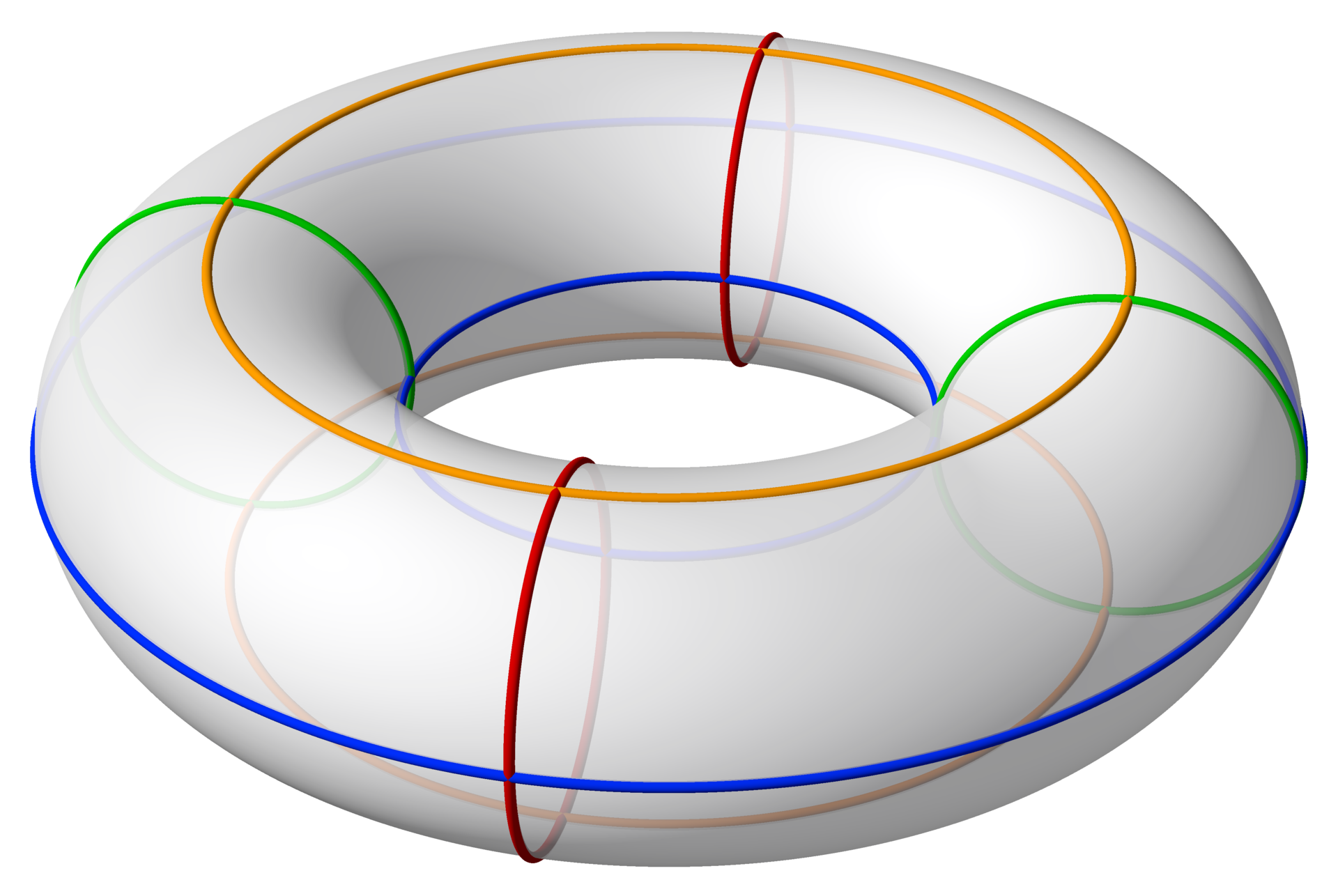
Fig 1. An example of Lie group, 2D Torus = $\mathsf{SO}(2)\times\mathsf{SO}(2)$, visualized
A Lie group $G$ is a differentiable manifold with an additional group structure (i.e. a way to define how two points multiply). Examples include the Special Orthongonal Group $\mathsf{SO}(n)$ (the set of $R \in \mathbb{R}^{n \times n}$ where $R^{\top}R = RR^{\top} = I, \det R = 1$), the Special Euclidean Group $\mathsf{SE}(n)=\mathbb{R}^n \rtimes \mathsf{SO}(n)$, the Special Unitary Group $\mathsf{SU}(n)$ (the set of $U \in \mathbb{C}^{n \times n}$ where $U^H U = U U^H = I, \det U = 1$), and their combinations (e.g., $n$-dim Torus). Lie group was a powerful notion classically used in physics (modeling continuous symmetry), control / robotics, and many other sciences and engineering domains. Generative modeling on Lie group also started attracting attention, and although that was rather recent, it already resulted in significant applications. For example:
- Protein design. To design new drugs, for example, one likes to creatively generate structures of proteins in 3D space. Such structures are often represented by backbone relative orientations between rigid functioning groups (roughly speaking), each relative orientation being an element of the special Euclidean group $\mathsf{SE}(3)$, which is a Lie group. Apart from this, in the protein structure there could also be torison angles modeled by products of $\mathsf{SO}(2)$, which is another Lie group.
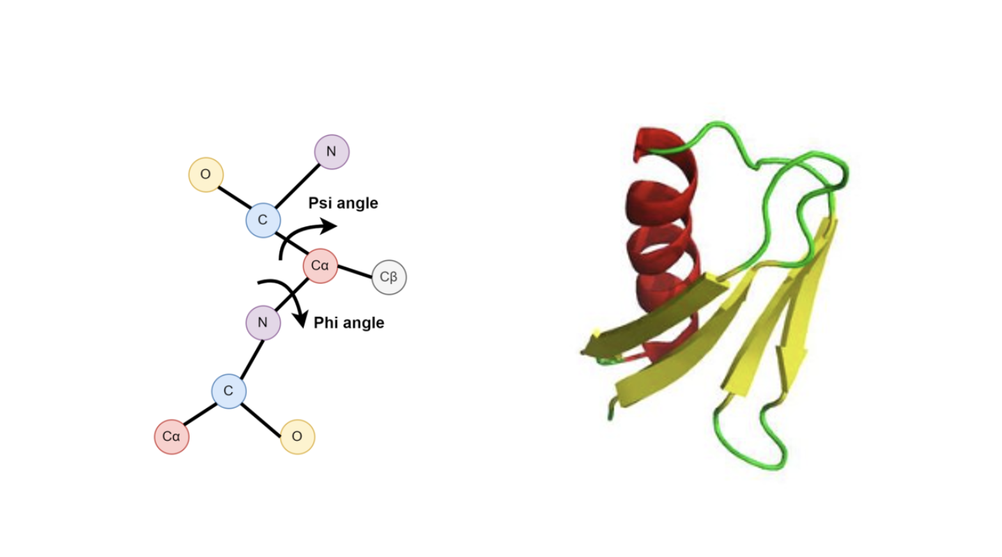
Fig 2. Examples of Lie group applications. Left: Torsion angles, each represented by an SO(2) element. Right: Protein backbone structures, connected via SE(3) elements
- Quantum computing. In quantum computing, the basic computing unit of quantum information is qubit. Similar to the use of circuits and logic gates in classical computation as operation on bits, quantum computation requires quantum logic gates and quantum circuits, which map qubits to some required values / realize some actions. Quantum circuits are unitary operations and thus elements of the Unitary Group $\mathsf{U}(N)$, which is another Lie group. While protein design already won a Nobel Prize, designing functioning quantum circuits via generative modeling on $\mathsf{U}(N)$ Lie group is an emerging but promising direction (see [Zhu+, ICLR’25] page 9-10 for preliminary work) .
To generalize diffusion models so that data on manifolds can be generatively modeled, multiple approximations are often needed. This is an important problem and therefore many great breakthroughs were made. For example, earlier, award-winning works include RSGM [De Bortoli+, NeurIPS’22], and RDM [Huang+, NeurIPS’22], and popular recent progress include a related, significant method known as RFM [Chen & Lipman, ICLR’24] (also award-winning). Different approaches make different approximations, but some common examples include: 1) naively extending the forward/backward dynamics to manifold would require Brownian motion on manifold, which cannot be exactly implemented in general due to the curved geometry, and thus need to be approximated (e.g., by discretization); 2) the exact score function $s(x,t)$ has its value living in the tangent fiber $T_{x}G$, but a neural network approximation may not live in $T_{x}G$, and as $x$ moves this space changes as well, which makes the accurate learning of score even more difficult.
When approximations are made, generation accuracy is compromised. That is why it is exciting to have a new approach that leverages the group structure to avoid approximations induced by curved geometry. The price to pay is, this method is less general and specializing only in Lie groups, which nevertheless already matter to important applications (see above). Let’s now describe this new method.
Trivialized Diffusion Model (TDM)
There is a line of recent developments on the mathematical foundations of machine learning on Lie groups. It started with a new approach based on variational optimization (see for example [Tao & Ohsawa, AISTATS’20], [Kong & Tao, NeurIPS’24], and [this blog post]), which was then generalized to a stochastic setting, resulting in an accelerated algorithm for sampling probability distribution on Lie group [Kong & Tao, COLT’24]. We will now leverage this sampling technique to go one step further, enabling accurate generative modeling on Lie group.
More precisely, [Kong & Tao, COLT’24] proved that the following dynamics converges to Gibbs distribution $Z^{-1}e^{-(U(g)+|\xi|^2)}dgd\xi$ regardless of the initial distribution under minimal condition,
\[\begin{cases} \dot{g} = g \xi, \\ \mathrm{d} \xi =-\gamma \xi \mathrm{d} t -T_{g} \mathsf{L}_{g^{-1}}(\nabla U(g)) \mathrm{d} t+ \sqrt{2\gamma}\mathrm{d} W^{\mathfrak{g}} \end{cases} \qquad (*)\]where $g(t)$ is an element of the Lie group $G$. This dynamics will be used as the forward dynamics of TDM.
A key benefit of such dynamics is that $\xi$ is a Euclidean variable thanks to a technique called left trivialization that led to this dynamics. In fact, expert readers may ask if this forward dynamics is some kind of underdamped Langevin equation. A short answer is, almost, but not exactly. More precisely, underdamped Langevin equation (or more rigorously put, kinetic Langevin eq.) in Euclidean space is
\[\begin{cases} \dot{q} = p, \\ \mathrm{d} p =-\gamma p \mathrm{d} t - \nabla U(q) \mathrm{d} t + \sqrt{2\gamma}\mathrm{d} W, \end{cases}\]where $q$ can be understood as the position of a particle moving in the Euclidean space, and $p$ is its time derivative, i.e. velocity/momentum (here we take mass=1 so these are roughly the same thing). However, the nontrivial construction of ($*$) is that, we no longer use $\dot{g}=p$ as a momentum variable, but instead use some nonlinear version $\xi$ given by $\dot{g}=g\xi$ instead (i.e. $\xi=g^{-1}p$). Physically, $\xi$ is angular momentum instead of linear momentum, and it makes all the difference.
In fact, while the usual velocity variable $\dot{g}$ belongs to the space $T_{g_t}G$, the trivialization technique utilizes the fact that $T_{g}G = g \cdot \mathfrak{g}$ and the trivialized momentum $\xi$ lives in something called the Lie algebra $\mathfrak{g} := T_{e}G$, which basically uses a left multiplication by $g^{-1}$ to pull all tangent vectors at $g$ back to the tangent space at $e$ (the identity element of the group). Consequently, unlike $T_g G$, which is a changing space as $g$ changes with time, the Lie algebra is a fixed vector space no matter how $g$ changes, which means $\xi$ essentially lives $\mathbb{R}^{d}$ at any time $t$. This is important, and notice that, with trivialized momentum, we only added additive, Euclidean noise to its dynamics. Algorithmically introducing the trivialized momentum $\xi$ not only bypasses the need for manifold Brownian motion, but greatly facilitates diffusion model, as we now demonstrate –
The relevance of ($*$) to diffusion model is, we can view $g$ as the “data” variable, while $\xi$ is an auxiliary variable artifically introduced to facilitate the design of a good algorithm.
For example, choosing $U(g)=0$ gives the following simple forward “noising” process,
\[\begin{cases} \dot{g_f} = g_f \xi_f, \\ \mathrm{d} \xi_f =-\gamma \xi_f \mathrm{d} t+ \sqrt{2\gamma}\mathrm{d} W^{\mathfrak{g}}, \end{cases}\]which converges to a simple distribution $Z^{-1}e^{-|\xi |^2/2} dg d\xi$ (product of uniform distribution on $G$ and Gaussian on $\mathfrak{g}$). We can initialize $g_f(0)$ as the data (distribution), and choose $\xi_f(0)$ to be any fully supported distribution, such as Gaussian (note it is unclear how to define Gaussian on a compact manifold, but here $\xi_f$ lives in a Euclidean space!) And then we just need a time reversal of this forward “noising” process. Once we have that, we can draw i.i.d. samples from $Z^{-1}e^{-|\xi |^2/2} dg d\xi$, use them as initial conditions and run the resulting time-reversed, backward “denoising” process. The $g$ component of their $T$-time evolutions will then be the generated samples.
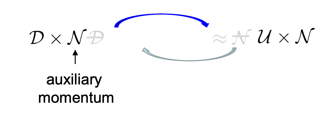
Fig 3. TDM maps between (data distribution, Gaussian) and (uniform, Gaussian) on the manifold $\mathsf{G}\times\mathfrak{g}$.
So we are just left with one key question, what is the backward dynamics of ($*$)? It is simply
\[\begin{cases} \dot{g_b} = -g_b \xi_b, \\ \mathrm{d} \xi_b = \gamma \xi_b \mathrm{d} t + 2 \gamma s(g_b, \xi_b, T-t) \mathrm{d} t+ \sqrt{2\gamma}\mathrm{d} B^{\mathfrak{g}} \end{cases}\]where the score function $s(g, \xi, t) = \nabla_{\xi} \log p(g, \xi, t)$ needed is simply an Euclidean derivative, only with respect to $\xi$, that is not geometrically constrained. This delightful feature avoids a major headache for generative modeling of manifold data! The fact that $s(g, \xi, t)$ is an Euclidean score in $\mathbb{R}^d$ implies that no effort is needed to ensure its value lives in $T_{g}G$, which is a space that changes with its input $g$. Instead, when learning the score function, you have the flexibility to use your favorite function parameterization, time-tested techniques in Euclidean diffusion models easily extrapolate, and there is no additional inaccuracy created by the curved geometry.
Readers short on time can stop here and still be able to get an impression of this new generative model.
One technical detail is: the inference process, i.e. the simulation of backward dynamics, requires initialization from $Z^{-1}e^{-|\xi |^2/2} dg d\xi$, and expert readers may ask if this can be done. The answer is yes. The core task is to sample from Haar measure $\propto dg$ (as sampling standard Euclidean Gaussian $\xi$ is trivial). Many methods exist, ranging from brutal force approaches such as to use the forward dynamics, or smart and efficient random linear algebra.
High accuracy inference by structure preserving integration
Another major source of inaccuracy of manifold diffusion models is the numerical simulation of backward dynamics during inference. The main reason is, when the space is curved, most generic time discretization methods will break the manifold structural constraints, even with a very small stepsize $h$.
For example, let’s consider the popular Euler-Maruyama numerical integrator of the backward equation,
\[\begin{cases} \hat g_b(t + h) = \hat g_b(t) - h \hat g_b(t) \hat \xi_b(t), \\ \hat \xi_b(t+h) = \hat \xi_b(t) + h \cdot \big(\gamma \hat \xi_b(t) + 2 \gamma s_{\theta}(\hat g_b(t), \hat \xi_b(t), T-t)\big) + \sqrt{2\gamma h} \cdot \epsilon \\ \epsilon \sim \mathcal{N}(0, I) \end{cases}\]We note that with this update scheme, even if we guarantee that the validness of the time $t$ state $\hat g_b(t), \hat \xi_b(t)$ by ensuring $\hat g_b(t) \in G$, $\hat \xi_b(t) \in \mathfrak{g}$, unfortunately we will find that $\hat g_b(t+h) \notin G$ as long as $h > 0$. Due to the non-trivial geometry of the Lie group, straightly following the tangent direction at each time step will always cause the state to leave the manifold. As a consequence, we often need to apply projection following the integration step to obtain a valid manifold element, which incurs additional computational cost and numerical errors.
But there is a way to numerically integrate the backward SDE and ensure the numerical solution remains satisfying its geometric constraint. More precisely, we can split its vector field as a sum of two vector fields, and build two dynamics respectively based on them:
\[\begin{array}{ccc} A_g: \Big\{ \begin{array}{ll} \dot{g_b} = -g_b \xi_b \\ \mathrm{d} \xi_b = 0 \end{array} & + & A_\xi: \Big\{ \begin{array}{ll} \dot{g_b} = 0 \\ \mathrm{d} \xi_b = \gamma \xi_b + 2\gamma s_{\theta}(g_b, \xi_b, T-t) \mathrm{d} t + \sqrt{2\gamma} \mathrm{d} B^{\mathfrak{g}} \end{array} \end{array}\]For $A_g$, since $\xi$ is not changing, the $g$-dynamics becomes a simple linear ODE, and its exact solution is thus analytically obtainable: we have $g_b(t+h) = g_b(t) \text{expm}(-h\xi_b)$. For $A_\xi$, instead $g_b$ is fixed, and the $\xi$-dynamics is essentially a linear SDE that is analytically solvable too because the nonlinear, neural network parametrized score term becomes a constant vector.
Due to the simplicity of the two sub-components of the backward equation, we can use a technique called Operator-Splitting to design a structure-preserving integrator for simulating the backward dynamics: instead of simutaneously update both $g_b$ and $\xi_b$, we update them by alternating the exact evolutions of $A_g$ and $A_\xi$.
A key benefit for this numerical simulation approach is that we guaranteed the manifold structural constraints at each update. This is because for Lie algebra elements $\xi_b$, $\exp(\xi_b)$ is an element in the Lie group, thus $g_b(t+h)$ always stays on the Lie group as $G$ is closed under group multiplication. On the other hand, $\xi_b$ always stays in the Lie algebra, and there’s no escape from that due to its isomorphism to Euclidean space. Thus, by considering this numerical scheme, we also successfully alleviate the approximation errors incurred by curved geometry in the inference stage.
Application
Let’s now see a demo of TDM’s applications. [Zhu+, ICLR’25] contains many more.
Generative Modeling of Protein Configurations via Angles
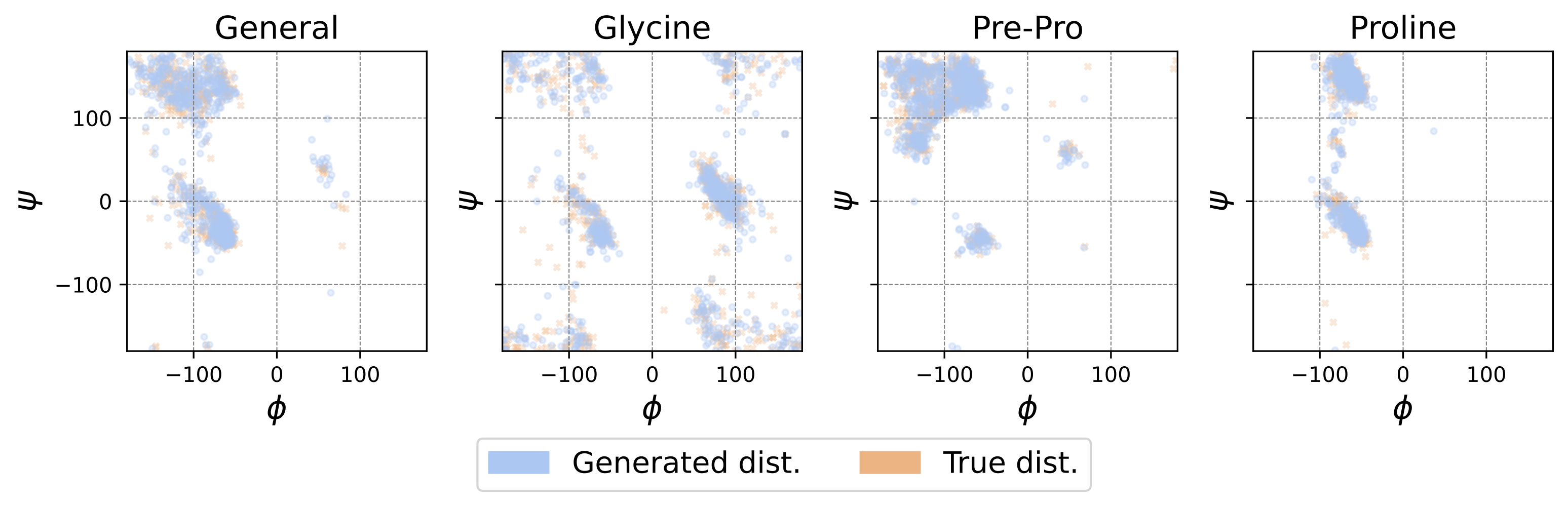
Here, we have many small peptides, of certain classes, as training data, and we’d like to generate configurations that fall into the same class. Each configuration is presented by angles and TDM is used to generate more configurations that are statistically alike. The fact that we can barely see two colors in the above scatter plot is due to very close matching of the generated distribution and the training data distribution, suggesting good accuracy for this highly multimodal task.
📝 How to Cite Me?
If you find this blog helpful, please cite the following paper:
@inproceedings{zhu2025trivialized,
title={Trivialized Momentum Facilitates Diffusion Generative Modeling on {L}ie Groups},
author={Yuchen Zhu and Tianrong Chen and Lingkai Kong and Evangelos Theodorou and Molei Tao},
booktitle={The Thirteenth International Conference on Learning Representations (ICLR)},
year={2025},
url={https://openreview.net/forum?id=DTatjJTDl1}
}
Comments
Join the discussion for this article on this ticket. Comments appear on this page instantly.